-
Notifications
You must be signed in to change notification settings - Fork 204
PICRUSt Tutorial with de novo Variants
Note this workflow is a work-in-progress and is still being altered. It is currently being tested and so should be used cautiously.
One drawback of using PICRUSt is that it restricts users to picking against OTUs in the Greengenes database. This is not ideal for several reasons including that a large proportion of OTUs are typically de novo and OTU picking is gradually being replaced by error correction approaches like DADA2 and deblur.
To get around this drawback the user can run the genome prediction steps of PICRUSt themselves (rather than having a pre-calculated supplied for reference OTUs).
If you are running this tutorial as part of EMBL-EBI's Metagenomics workshop then the tutorial files should already be on your computer. You can copy the zipped folder to the Desktop, unzip it, and enter the folder to get started.
cd ~/Desktop
cp ~/Documents/picrust_tutorial_Oct2017.zip ~/Desktop
unzip picrust_tutorial_Oct2017.zip
cd picrust_tutorial_Oct2017
Otherwise you can download the tutorial files by replacing the cp command above with the below wget command.
wget http://kronos.pharmacology.dal.ca/public_files/tutorial_datasets/picrust_tutorial_Oct2017.zip
In the picrust_tutorial_Oct2017 directory you will see output files from the DADA2 pipeline and required files that will be used for the genome prediction steps.
Before proceeding with this workflow you will need to activate the qiime1 anaconda environment.
source ~/anaconda2/bin/activate qiime1
Concatenate study and reference 16S rRNA gene sequences into a single file.
cat dada2_out/seqtab.fasta img_gg_starting_files/gg_13_5_img_subset.fasta > study_seqs_gg_13_5_img_subset.fasta
Align all sequences to full Greengenes reference using PyNAST ~ 1m30s:
align_seqs.py -e 90 -p 0.1 -i study_seqs_gg_13_5_img_subset.fasta -o study_seqs_gg_13_5_img_subset_pynast
Filter alignment:
filter_alignment.py -i study_seqs_gg_13_5_img_subset_pynast/study_seqs_gg_13_5_img_subset_aligned.fasta -o study_seqs_gg_13_5_img_subset_pynast
Run fasttree with topology constraints for reference sequences, ~1min
export OMP_NUM_THREADS=9
FastTreeMP  -nt -gamma -fastest -no2nd -spr 4 -constraints img_gg_starting_files/99_otus_IMG_pruned_no_names_constraint.txt < study_seqs_gg_13_5_img_subset_pynast/study_seqs_gg_13_5_img_subset_aligned_pfiltered.fasta > study_seqs_gg_13_5_img_subset.tre
Start by formatting input tree and trait table.
format_tree_and_trait_table.py -t study_seqs_gg_13_5_img_subset.tre -i img_gg_starting_files/gg_13_5_img_16S_counts.txt -o format/16S

format_tree_and_trait_table.py -t study_seqs_gg_13_5_img_subset.tre -i img_gg_starting_files/img_400_ko.tab -o format/KO -m img_gg_starting_files/gg_13_5_img_fixed.txt
Run ancestral state reconstruction steps for 16S rRNA gene counts.
ancestral_state_reconstruction.py -i format/16S/trait_table.tab -t format/16S/pruned_tree.newick -o asr/16S_asr_counts.tab -c asr/asr_ci_16S.tab
You could also run this command to run ASR for the KO table. This command takes ~24 minutes so we have made the output files available in img_gg_starting_files/KO_asr_precalc. Again you do not need to run the below command.
ancestral_state_reconstruction.py -i format/KO/trait_table.tab -t format/KO/pruned_tree.newick -o asr/KO_asr_counts.tab -c asr/asr_ci_KO.tab
Get names of dada2 variants
grep ">seq" dada2_out/seqtab.fasta | tr -d ">" | tr "\n" "," > study_ids.txt
Run predict traits:
predict_traits.py -i format/16S/trait_table.tab -t format/16S/reference_tree.newick -r asr/16S_asr_counts.tab -o predicted/16S_precalculated.tab -a -c asr/asr_ci_16S.tab -g "$(< study_ids.txt)"

predict_traits.py -i format/KO/trait_table.tab -t format/KO/reference_tree.newick -r img_gg_starting_files/KO_asr_precalc/KO_asr_counts.tab -o predicted/KO_precalculated.tab -a -c img_gg_starting_files/KO_asr_precalc/asr_ci_KO.tab -g "$(< study_ids.txt)"
echo "" >> predicted/KO_precalculated.tab
cat img_gg_starting_files/metadata/precalc_meta >> predicted/KO_precalculated.tab
normalize_by_copy_number.py -i dada2_out/seqtab_tax_rarified.biom -c predicted/16S_precalculated.tab -o seqtab_tax_rarified_norm.biom

predict_metagenomes.py -i seqtab_tax_rarified_norm.biom -c predicted/KO_precalculated.tab -o seqtab_tax_rarified_norm_ko.biom

categorize_by_function.py -i seqtab_tax_rarified_norm_ko.biom -o seqtab_tax_rarified_norm_ko_l3.biom -c KEGG_Pathways -l 3
Run metagenome contributions:
metagenome_contributions.py -i seqtab_tax_rarified_norm.biom -l K08602,K03699 -o metagenome_contributions.txt -c predicted/KO_precalculated.tab
Plot stacked barcharts of metagenome contributions:
plot_metagenome_contributions.R --input metagenome_contributions.txt --output K03699_contrib.pdf --function_id K03699 --rank Genus
You should see this figure:

Convert to STAMP format.
biom_to_stamp.py -m "KEGG_Description" seqtab_tax_rarified_norm_ko.biom > seqtab_tax_rarified_norm_ko.spf
biom_to_stamp.py -m "KEGG_Pathways" seqtab_tax_rarified_norm_ko_l3.biom > seqtab_tax_rarified_norm_ko_l3.spf
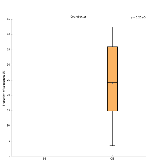
The top KO after FDR multiple-test correction as barplot:

The top KEGG pathway after FDR multiple-test correction as boxplot:

- Please feel free to post a question on the Microbiome Helper google group if you have any issues.
- General comments or inquires about Microbiome Helper can be sent to [email protected].