Statistics and stochastic calculus for Markov processes in continuous time, include univariate and multivariate stochastic processes such as stochastic differential equations or diffusions (SDE's) or Levy processes.
I am personally interested in doing Bayesian inference on discretely observed diffusion processes, but this package is written to be of general use and contributions are welcome. Specifically for our code for parameter inference for diffusion processes from discrete data or passage times, check out the dependent package BridgeSDEInference.jl. The statistical method relies a lot on simulating conditional diffusions (so called "difffusion bridges"). See ./example/tutorial.jl for a more general introduction into working with this package.
- Define and simulate diffusion processes in one or more dimension
- Continuous and discrete likelihood using Girsanovs theorem and transition densities
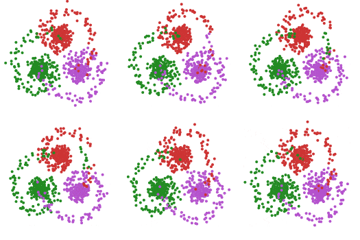
- Monte Carlo sample diffusion bridges, diffusion processes conditioned to hit a point v at a prescribed time T
- Brownian motion in one and more dimensions
- Ornstein-Uhlenbeck processes and Ornstein-Uhlenbeck bridges
- Bessel processes
- Gamma processes
- Inhomogenous poisson process
- Basic stochastic calculus functionality (Ito integral, quadratic variation)
- Euler-Scheme and implicit methods (Runge-Kutta)
- Levy-driven SDEs
- Continuous-discrete filtering for partially observed diffusion processes
The layout/api was originally written to be compatible with Simon Danisch's package FixedSizeArrays.jl. It was refactored to be compatible with StaticArrays.jl by Dan Getz.
Some SDE and ODE solvers in Bridge are accessible with the JuliaDiffEq common interface via BridgeDiffEq.jl.
The example programs in the example/ directory have additional dependencies: ConjugatePriors and a plotting library.
The key objects introduced are the abstract type ContinuousTimeProcess{T} parametrised by the state space of the path, for example T == Float64 and various structs suptyping it, for example Wiener{Float64} for a real Brownian motion. These play roughly a similar role as types subtyping Distribution in the Distributions.jl package.
Secondly, the struct
struct SamplePath{T}
    tt::Vector{Float64}
    yy::Vector{T}
    SamplePath{T}(tt, yy) where {T} = new(tt, yy)
end
serves as container for sample path returned by direct and approximate samplers (sample, euler, ...).
tt is the vector of the grid points of the simulation and yy the corresponding vector of states.
Help is available at the REPL:
help?> GammaProcess
search: GammaProcess LocalGammaProcess VarianceGammaProcess
GammaProcess |
|---|
A GammaProcess with jump rate ν(x) = γ x⁻¹ exp(-λ x), Here Examples
|
Pre-defined processes defined are
Wiener, WienerBridge, Gamma, LinPro (linear diffusion/generalized Ornstein-Uhlenbeck) and others.
It is also quite transparent how to add a new process:
using Bridge
using Plots

# Define a diffusion process
struct OrnsteinUhlenbeck  <: ContinuousTimeProcess{Float64}
    β::Float64 # drift parameter (also known as inverse relaxation time)
    σ::Float64 # diffusion parameter
end

# define drift and diffusion coefficient of OrnsteinUhlenbeck
Bridge.b(t, x, P::OrnsteinUhlenbeck) = -P.β*x
Bridge.σ(t, x, P::OrnsteinUhlenbeck) = P.σ

# simulate OrnsteinUhlenbeck using Euler scheme
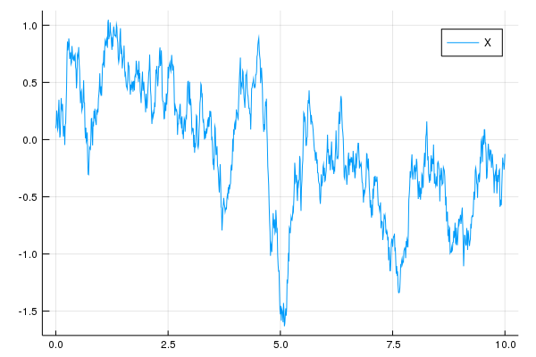
W = sample(0:0.01:10, Wiener())
X = solve(EulerMaruyama(), 0.1, W, OrnsteinUhlenbeck(2.0, 1.0))
plot(X, label="X")
# Levy (Difference-Gamma process) driven OrnsteinUhlenbeck
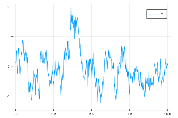
Z = sample(0:0.01:10, GammaProcess(100.0,10.0))
Z.yy .-= sample(0:0.01:10, GammaProcess(100.0,10.0)).yy
Y = solve(EulerMaruyama(), 0.1, Z, OrnsteinUhlenbeck(2.0, 1.0))
plot(Y, label="Y")See the documentation for more functionality and issue #12 (Feedback and Contribution) for coordination of the development. Bridge is free software under the MIT licence. If you use Bridge.jl in a closed environment I’d be happy to hear about your use case in a mail to [email protected] and able to give some support.
F. v. d. Meulen, M. Schauer: Bayesian estimation of discretely observed multi-dimensional diffusion processes using guided proposals. Electronic Journal of Statistics 11 (1), 2017, doi:10.1214/17-EJS1290.
M. Schauer, F. v. d. Meulen, H. v. Zanten: Guided proposals for simulating multi-dimensional diffusion bridges. Bernoulli 23 (4A), 2017, doi:10.3150/16-BEJ833.


