QSPD

QSPD is used to solve the rate equations to obtain the quantum states population dynamics.

Introduction

QSPD uses Einstein rate equation model to construct the rate equations, and solve them to get the population dynamics.
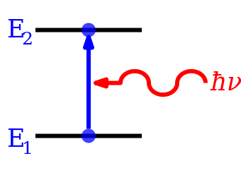
The simplest case is a 2-level system namely there're two states with different energies in the system. According to the model, three types of transition can happen.

1. Absorption process - absorbing a photon to go to the higher-energy level

   

2. Spontaneous emission process

   

3. Stimulated emission process

   

The Einstein rate equation then can be written as:

where is the population fraction in state i. The system of equations includes the rovibronic and hyperfine states of interest. The initial population was assumed to be thermal with a temperature of 300 K. and are the energy densities of the blackbody radiation and laser. and are the spontaneous emission and stimulated emission Einstein coefficients, respectively. The subscripts i and j are used to indicate the quantum state. The states are sorted in the ascending order by the state energy. Therefore, when i < j, the energy of state i is less than state j.

Usage

1. Prepare necessary files for constructing the rate equation. To construct the rate equations, you need the following .csv files.

   1. the transition energy matrix, TransE[i,j] = StateEnergy[i]-StateEnergy[j]. The example file is AlH+\_v1_TransitionEnergy_Threshold-6.csv in the repository.
   2. the oscillator strength matrix The example file is AlH+\_v1_OscillatorStrength_Threshold-6.csv in the repository
   3. the array of state degeneracies. The example file is AlH+\_v1_J_degeneracy_sort_by_Energy_Threshold-6.csv

2. Open Quantum_States_Population_Dynamics_Simulation.py. Change the paths of the required files in step 1 in it, and run. The state population changing with time will be saved to a .csv file. The dynamics of the states with the poulation > 5% at the end of the simulation time will be saved as a .pdf plot.

Note 1:

the states are sorted by the state energy in the ascending order.

Note 2:

If you have a Pgopher file constructed, you can change the unit of the transition strength in Pgopher to oscillator strength and export a transition line file from Pgopher. After you have the exported file, use the file TransItion_Info_from_Pgopher.ipynb to generate the three required files above. Example pgopher output file: AlH+_A-X_transition_v1_0Gauss_Random_JMax50_Threshold-6.csv