Focont

Static output feedback and fixed order controller design package for Python

Static output feedback (SOF)

SOF is the simplest feedback controller structure. More precisely, it redirects the system output to the system input after multiplying by a constant gain matrix. You can find brief information about SOF in this page.

The algorithm implemented in this package can calculate a stabilizing SOF gain which also minimizes the $\mathcal{H}_2$ norm of the closed loop system. The resulting controller is comparable to the result obtained by linear quadratic regulators (LQR) with respect to the impulse response energy of the closed loop system.

However, this algorithm works when some sufficient conditions are satisfied. If the problem parameters (listed below) is not appropriate, the algorithm fails and prints an error message. Please see the article, and the PhD thesis, for detailed information and analysis.

The algorithm is mainly developed for discrete time systems, but it may also compute similar SOF gains for continuous time systems when this algorithm is applied to the zero-order hold (ZOH) discretized versions with a sufficiently large sampling frequency.

Furthermore, the algorithm can be used to calculate fixed-order controllers. Please, check tests for examples and docs for detailed information.

Installation

python3 -m venv venv
source venv/bin/activate
pip install -e '.[dev]'
pytest

Also,

It can be installed via pip from pypi.

pip install focont

Example

Consider this highly simplified real life example below which is a naively discretized version of the ideal Newton motion equations. It is a model of a ball's motion on an inclined plane.

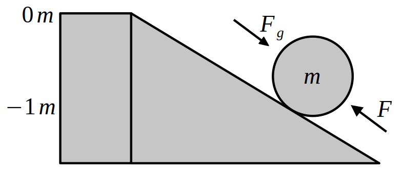
In the model, the top of plane is assumed to be the origin and force $F$ pushes the ball to move it to the origin. The force $F_g$ is the effect of gravity and there is a mild friction which is damping the velocity of the ball. The system parameters are chosen in a way to make numbers simpler to write.

$$ p_{t+1} = p_t + 0.01 p_t + 0.1 v_t $$

where $t \in \{ 0, 1, \dots \}$ is the discrete time instants, $p_t$ is the vertical position $v_t$ is the velocity and is accumulated in $p_t$. The term $+0.01 p_t$ is a result of constant $F_g$ force.

$$ v_{t+1} = v_t - 0.01 v_t + F_t $$

where $v_t$ is the velocity. The second term is damping and the last term is the force that pushes the ball upwards. Finally, it is assumed that the sum of vertical position and velocity can be measured.

$$ y_t = p_t + v_t $$

With this information, the system matrices can be written as

$$ x_{t+1} = Ax_t + Bu_t, ~~~ y_t = Cx_t $$

where

$$ x_t = \begin{bmatrix} p_{t+1} \\ v_{t+1} \end{bmatrix} ~~ A = \begin{bmatrix} 1.01 & 0.1 \\ 0 & 0.99 \end{bmatrix} ~~ B = \begin{bmatrix} 0 \\ 1 \end{bmatrix} ~~ C = [ 1 ~~ 1 ] $$

Problem:

Calculate a static output feedback (SOF) gain $K$ that minimizes

$$ J = \sum_{t=0}^{\infty} p_t^2+F_t^2 $$

where force is a function of measurment

$$ F_t = Ky_t $$

In other terms, how can I use the measurment $y_t$ to move the ball to the top as quickly as possible while spending as low as energy possible. The script below solves this problem.

from focont import foc, system

def main():
    A = [
        [ 1.01, 0.10 ],
        [ 0.00, 0.99 ],
    ]
    B = [
        [ 0 ],
        [ 1 ],
    ]
    C = [ [ 1, 1 ] ]
    Q = [
        [ 1, 0 ],
        [ 0, 0 ],
    ]
    R = [ [ 1 ] ]
    data = { "A": A, "B": B, "C": C, "Q": Q, "R": R }

    pdata = system.load(data)
    foc.solve(pdata)
    foc.print_results(pdata)

if __name__ == "__main__":
    main()

Prints out:

 Progress:      10%, dP=0.4662574448312318
 Iterations converged, a solution is found
- Stabilizing SOF gain:
[[-0.6147]]
- Eigenvalues of the closed loop system:
[0.8907 0.4946]
 |e|:
[0.8907 0.4946]

Meaning that, $K$ must be chosen as $K=-0.6147$. For this problem, the closed loop system is stable when $-2 < K < -0.01$ according to the result of Octave's rlocus method. When the cost $J$ is calculated for $K$ in this interval the plot below is obtained.

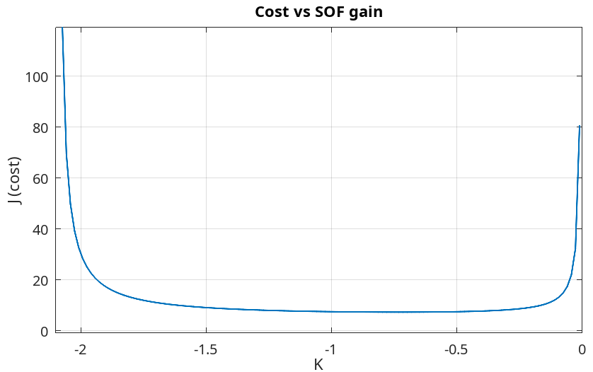
In this plot, the minimum cost is $7.35$ when $K=-0.7306$ which is close to the cost $7.38$ at $K=-0.6147$.

Let us modify the cost function and attach a higher weight to the consumed energy. Meaning that, we do not care much about how quickly the ball is transported but we want to spend less energy.

$$ J = \sum_{t=0}^{\infty} p_t^2+10 F_t^2 $$

In this case, the SOF gain $K=-0.2717$ is obtained. The plot below shows the differences between $p_t, v_t$ and $u_t$ for both SOF gains $K$.

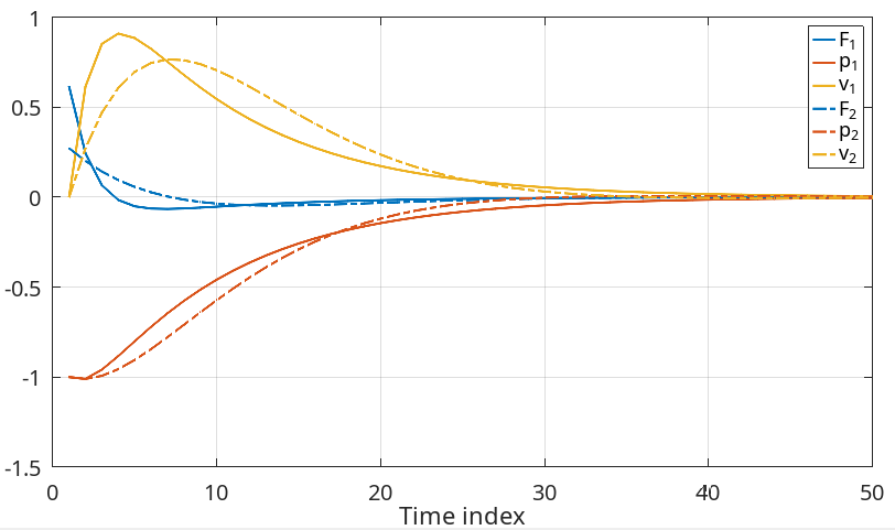
The dashed lines are obtained when the consumed energy is largely penalized in the cost function. As it can be seen, it gets closer to the origin slower, but consumed energy (blue) is smaller.